Association of Republican partisanship with US citizens' mobility during the first period of the COVID crisis | Scientific Reports

Data

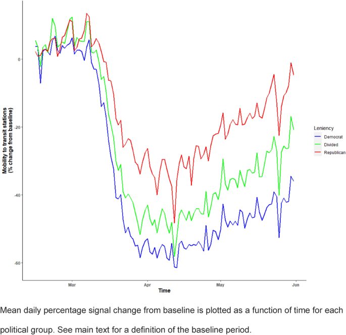
Outcome variable (mobility to transit stations)

We used the Google COVID-19 Community Mobility Reports database to extract state-wise daily percentage change in mobility to transit stations²³. This database has been used extensively to assess various interventions during the pandemic. It provides longitudinal data for six particular categories of mobility data: (1) transit stations; (2) retail and recreation places; (3) workplaces; (4) groceries and pharmacies; (5) residential places; (6) parks. Observations are based on cellular phone, laptop and tablet signals. Specifically, the data shows how visits and time spent in the above places change compared to so-called “baseline days”. For each day of the week, the baseline day is the median value from the 5‑week period Jan 3–Feb 6 2020 (i.e. before the pandemic hit the US, hence before restrictions on movement) for a specific location and a specific mobility category. For each day, an integer value gives the percent change in mobility (positive or negative) compared to that same day during that 5-week period (Jan 3–Feb 6).

In the current study, we chose mobility to transit stations as our main outcome of interest and used other measures in our sensitivity analysis²⁴. We chose to restrict our time series to the period from February the 15th 2020 (start date of the database) till May the 31th 2020. The latter is often taken as the end of the first wave of the pandemic. In total, our time series amounts to 107 days. Overall, our data comprised N = 51 states × 107 days = 5457 observations. There were no missing values.

Political orientation

Each state’s political orientation was defined as each state trifecta as of 2020 (Democratic vs. divided vs. Republican) and retrieved from the ballotpedia website²⁵. A state government trifecta occurs when either the Republican or the Democratic party holds the governorship and a majority in both chambers of a state’s legislature. States where neither party holds trifecta control are reported to be “divided”. In the Supplementary Materials 1, we provide a list and a map of US states according to their political affiliation.

Stringency of anti-COVID measures

For each state and each day, a measure of the stringency of anti-COVID interventions was extracted from the Oxford COVID-19 Government Response Tracker (OxCGRT)²⁶. In short, the OxCGRT provides a measure of stringency on a scale from 0 to 100, publicly available on GitHub²⁷. This measure is based on a summary of seven indicators on policies regarding social isolation and confinement, including school, workplace, and public transport closures, public events cancellations, stay at home requirements, and restrictions on gatherings and internal movement. Data is collected from publicly available sources such as news articles and government press releases and briefings. Each indicator measures the stringency of each policy or intervention on an ordinal scale of severity or intensity (from no measures taken to simple recommendations and implementation of the policy). Note that OxCGRT measures for US states do not include federal policies that apply to the country as a whole (e.g., international travel bans).

We reasoned that the effect of anti-COVID measures would be expected on citizens’ mobility on the day they were introduced, as in²⁸, therefore we did not include any lags in the “Stringency” time series.

Cumulative number of COVID deaths

We used the daily cumulative number of COVID deaths in each state as a reflection of the amount of risks due to COVID perceived daily by citizens in each state¹⁹. Indeed, we reasoned that a great marginal increase in the number of COVID-related deaths would inform citizens that the current status of the pandemic may be dangerous. And in turn, a large (negative) effect of the number of COVID deaths on mobility would suggest that citizens take great precautions against the virus by not going out. For each state and each day, the cumulative number of confirmed COVID-related deaths was extracted from the Oxford COVID-19 Government Response Tracker, and lagged by one day²⁷. Note that for the purpose of our research question, we indeed reasoned that an optimal way to model the impact of COVID deaths on citizens’ mobility would be to use the raw number of deaths rather than rates. This is because our hypothesis relies on the impact of COVID deaths on mobility via people’s perceptions of the danger to go out due to an increased number of COVID deaths. In that sense, we hypothesized that a raw number would be more meaningful to people than a (relatively small) rate.

Temperature

We included a climate variable in our statistical model as we reasoned that climate might confound the relationship between COVID deaths and mobility. We retrieved the mean temperature (in degrees Fahrenheit) of each state’s capital city for each day of our time series from the wunderground website²⁹.

Analysis

Main analysis

We specified multivariate linear models using directed acyclic graphs to include variables that appeared to determine mobility to transit stations (Supplementary Materials 2). Specifically, we fit our time series of the mobility to transit stations according to the following linear equation:

$$beginaligned Mobility_sd = & beta_0 + beta_1 Stringency_sd + beta_2 Stringency_sd *Republican_s \ & + beta_3 Deaths_sd + beta_4 Deaths_sd *Republican_s \ & + beta_5 Temp_sd + beta_6 Temp^2_sd \ & + beta_7 Trend_d *Republican_s \ & + theta_s + delta_d + epsilon_sd \ endaligned$$

where:

(Mobility_sd ) is the percent signal change from baseline in mobility to transit station, for state (s) at day (d);

(Stringency_sd) is a measure of the stringency of anti-COVID interventions, for state (s) at day (d);

(Republican_s) is an indicator of Republican partisanship for each state (s). For the purpose of our main analysis, we define a crude index of Republican partisanship according to each state’s trifecta, where Democratic states would be affiliated the value of 0, divided states the value of 1, and Republican states the value of 2;

(Deaths_sd) is the number of COVID deaths (cumulative) for state (s) at day (d);

(Temp_sd) and (Temp^2_sd) are measures of the mean temperature of each state (s) capital city at day (d) (raw and squared terms, respectively);

(Trend_d) indicates temporal count, taking the value (d) at day (d). Note that we also tested a model including a non-linear, quadratic temporal trend, which we subsequently decided to remove as it was non-significant;

(beta _i) indicates the parameter estimate of the respective regressor (i). We were specifically interested in (beta _2) and (beta _4), which represent the effect of anti-COVID stringency measures and cumulative COVID Deaths on citizens’ mobility moderated by Republican partisanship, respectively. We were also interested in (beta _7), which represents the effect of Republican partisanship on mobility over time;

(theta _s) represent states fixed effects for each state (s). States fixed effects are “omitted” and unobserved state-level time-invariant factors that distinguish US states and that could bias our statistical estimates of interest. These would be confounders in the relationship between treatments and outcome, i.e. factors that may influence anti-COVID measures and/or the cumulative number of COVID deaths, as well as citizens’ mobility. Such factors might be (but are not restricted to): population-level risk preferences³⁰, general level of trust to politicians and healthcare systems³¹, culture, ethnicity and religion, population density, percentage of urban population, share of population aged 65 or older, average household size, unemployment rate, income per capita and income inequality^32,33,34, percentage of the population with risk factors for COVID-19 (such as obesity or cardio-vascular disease), state’s physician rate;

(delta _d) represent days fixed effect for each day (d). Days fixed effects model time-varying state-invariant factors that may confound our main relationships of interest. In short, these would be represented by nationwide daily variability in movement, for instance due to national holidays, weekend days, vacation periods, economic downturns, or nationwide weather patterns;

(epsilon _sd) is the model residual for state (s) at day (d).

Because policy stringency and the number of COVID deaths likely correlate with the time variable, the presence of multicollinearity among variables included in the model was investigated. The variance inflation factor was below 7.5 for each regressor, and below 5 for our three regressors of interest. When we further scaled the temperature variable (linear and quadratic terms), the variance inflation factor was below 5 for each regressor, without any change in the mean coefficient value for each parameter of interest ((beta _2),(beta _4) and (beta _7)).

Cluster robust standard errors were estimated to account for the correlation of data within each state. Note that we did not include a main effect of Republican partisanship, nor a single linear temporal trend in our statistical model as these would be collinear with states and days fixed effects, respectively.

Event-studies

We performed additional analysis where variables Stringency, Deaths and Trend were discretized. Specifically, Stringency, Deaths and Trend were discretized into 10 categorical bins, such that each bin contained enough data to perform additional regression analyses (see Supplementary Materials 4 for a table summarizing the number of observations contained in each bin for each political group). Doing so, the chances of data sparsity were reduced, which improves the interpretability of our results. Another reason why we performed these additional analyses is that they provide better insights on the effect modification of Stringency, Deaths and Trend by Republican partisanship, because discretization allows better visualization of subtle non-linear effects.

We specified the following linear equation:

$$beginaligned Mobility_sd = & beta_0 + beta_1 Stringency_sd + mathop sum limits_i = 1^10 alpha_i left( BinStringency_sdi *Republican_s right) \ & + beta_3 Deaths_sd + mathop sum limits_j = 1^10 gamma_j left( BinDeaths_sdj *Republican_s right) \ & + beta_5 Temp_sd + beta_6 Temp^2_sd \ & + mathop sum limits_k = 1^10 lambda_k left( BinTrend_sdk *Republican_s right) \ & + theta_s + delta_d + epsilon_sd \ endaligned$$

where (BinStringency_sdi), (BinDeaths_sdj) and (BinTrend_sdk) take the value of 1 if (BinStringency_sdi), (BinDeaths_sdj) and (BinTrend_sdk) correspond to the value of (i,j,k), respectively.

(alpha _1, gamma _1 , lambda _1) are the reference coefficients and are set to 0.

(alpha _i, gamma _j , lambda _k) therefore indicates the effects of Republican partisanship on mobility at each bin (i,j,k) comparatively to that at bins (i=1, j=1, and ,k=1) for Stringency, Deaths and Trend, respectively.

We then reported so-called “event-study plots” to illustrate the effect of each discretized variable, modified by Republican partisanship, on the outcome.

Sensitivity analysis

We ran the following sensitivity analysis to check that subtle changes in measurement would not invalidate our conclusions.

Outcome variable

Here, we substituted mobility to transit stations to that of other places where signals were recorded in the Google COVID-19 Community Mobility Reports database: retail and recreation places, workplaces, groceries and pharmacies, residential places, and parks.

We hypothesized that our estimates of interest would not substantially change as compared to those obtained with mobility to transit stations when outcome variables were mobility to retail and recreation places, workplaces, and groceries and pharmacies. For residential places, we hypothesized that estimates would be of an opposite sign than those obtained with transit stations. Finally, we hypothesized that estimates would be non-significant for mobility to parks, as we reasoned that these would be much less impacted by subtle exposure changes.

Measurement of Republican partisanship

Here, we changed our strategy for measurement of Republican partisanship. Using data from the Pew Research Center, we differentiated states in terms of their percentage of voters for the Republican candidate at the 2016 presidential elections (former President Trump), rather than a rough differentiation of their political group as we did in the main analysis (Democratic vs. divided vs. Republican states) ³⁵.

Measurement of risk perception

We re-ran our main analysis using cumulative COVID cases instead of cumulative COVID deaths as a measure of perception of COVID risk.

Accounts of temporality

We first tested a model taking into account a specific correlation structure of the error term, as sequences of non-seasonal Autoregressive Moving Average (ARMA) of daily values for each state, with p = 1 lag.

Second, to test whether our results were robust to a longer period of analysis, we reproduced our event-study plots (aming to illustrate the effect of each variable of interest, modified by Republican partisanship) over a longer period of analysis (till the end of February 2021 rather than end of May 2020).

Analyses were performed R version 4.0 and packages daggity, fixest and nlme.

Published on The Perfect Enemy at https://bit.ly/3POFtwy.

Julio Marchi © Speaks Out Network

Search This Blog